Query and analyze spatial data
After having created a SpatialData collection, we briefly discuss how to query and analyze spatial data.
import lamindb as ln
import bionty as bt
import squidpy as sq
import scanpy as sc
import spatialdata_plot
import warnings

warnings.filterwarnings("ignore")

ln.track(project="spatial guide datasets")
Query by data lineage
Query the transform, e.g., by key:
transform = ln.Transform.get(key="spatial.ipynb")
transform
Query the artifacts:
ln.Artifact.filter(transform=transform).df()
Query by biological metadata
Query all visium datasets.
all_xenium_data = ln.Artifact.filter(experimental_factors__name="10x Xenium")
all_xenium_data.df()
Query all artifacts that measured the “celltype_major” feature:
# Only returns the Xenium datasets as the Visium dataset did not have annotated cell types
feature_cell_type_major = ln.Feature.get(name="celltype_major")
query_set = ln.Artifact.filter(feature_sets__features=feature_cell_type_major).all()
xenium_1_af, xenium_2_af = query_set[0], query_set[1]
xenium_1_af.describe()
xenium_1_af.view_lineage()

xenium_2_af.describe()
xenium_2_af.view_lineage()

Analyze spatial data
Spatial data datasets stored as SpatialData objects can easily be examined and analyzed through the SpatialData framework, squidpy, and scanpy:
xenium_1_sd = xenium_1_af.load()
xenium_1_sd
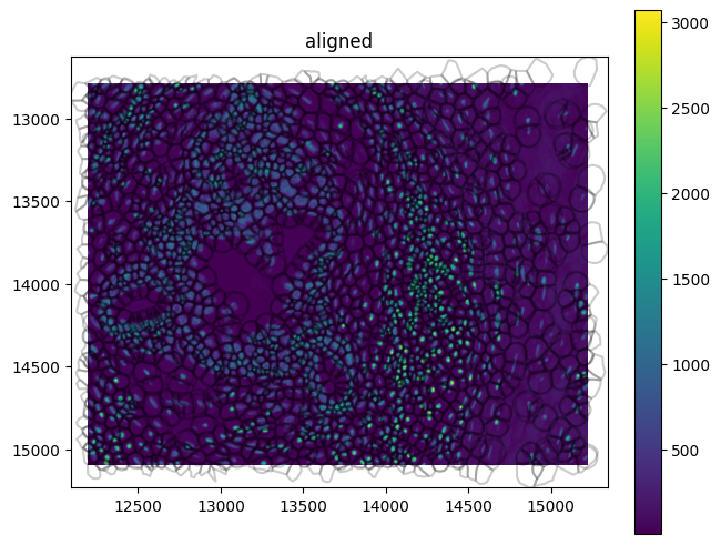
Use spatialdata-plot to get an overview of the dataset:
xenium_1_sd.pl.render_images(element="morphology_focus").pl.render_shapes(
    fill_alpha=0, outline_alpha=0.2
).pl.show(coordinate_systems="aligned")
For any Xenium analysis we would use the AnnData object, which contains the count matrix, cell and gene annotations.
It is stored in the spatialdata.tables slot:
xenium_adata = xenium_1_sd.tables["table"]
xenium_adata
xenium_adata.obs
Calculate the quality control metrics on the AnnData object using scanpy.pp.calculate_qc_metrics:
sc.pp.calculate_qc_metrics(xenium_adata, percent_top=(10, 20, 50, 150), inplace=True)
The percentage of control probes and control codewords can be calculated from the obs slot:
cprobes = (
    xenium_adata.obs["control_probe_counts"].sum()
    / xenium_adata.obs["total_counts"].sum()
    * 100
)
cwords = (
    xenium_adata.obs["control_codeword_counts"].sum()
    / xenium_adata.obs["total_counts"].sum()
    * 100
)
print(f"Negative DNA probe count % : {cprobes}")
print(f"Negative decoding count % : {cwords}")
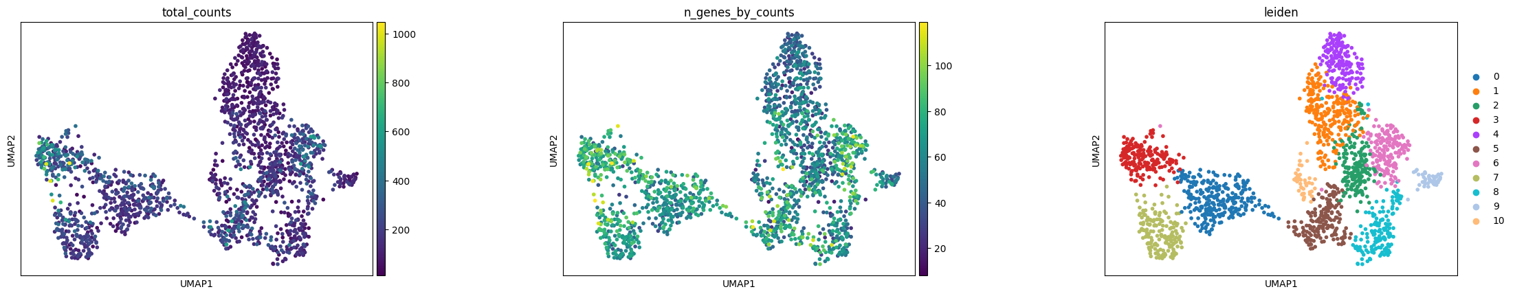
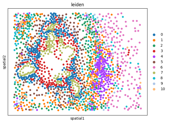
Visualize annotation on UMAP and spatial coordinates:
xenium_adata.layers["counts"] = xenium_adata.X.copy()
sc.pp.normalize_total(xenium_adata, inplace=True)
sc.pp.log1p(xenium_adata)
sc.pp.pca(xenium_adata)
sc.pp.neighbors(xenium_adata)
sc.tl.umap(xenium_adata)
sc.tl.leiden(xenium_adata)
sc.pl.umap(
    xenium_adata,
    color=[
        "total_counts",
        "n_genes_by_counts",
        "leiden",
    ],
    wspace=0.4,
)
sq.pl.spatial_scatter(
    xenium_adata,
    library_id="spatial",
    shape=None,
    color=[
        "leiden",
    ],
    wspace=0.4,
)
For a full tutorial on how to perform analysis of Xenium data, we refer to squidpy’s Xenium tutorial.
ln.finish()